Though much of our educational focus centers on how to arrive at a buy or sell decision, our analysis doesn’t end at the moment we send in an order ticket. Instead, as an actively-managed portfolio, we analyze our performance monthly, quarterly, and annually, in order to determine how well our portfolio is performing relative to our benchmark, the S&P 500.

On the most basic level, it is important to realize our portfolio is very different from the S&P 500 in terms of its allocation. We typically hold under 50 stocks across the 10 sectors, meaning around 450 stocks from our benchmark have no representation in our portfolio. For each individual stock in our portfolio, we can calculate an active weight as follows, where value is defined as the number of shares held multiplied by the market price:

Active weights can be either positive or negative. If an active weight is positive, we are overweight, and if it is negative, we are underweight. We would prefer to be overweight in positions which we expect to do well in the future, and underweight in those stocks which we expect to perform poorly. If we match this goal, we would earn larger gains and suffer smaller losses than would someone who buys an S&P 500 index fund, which is just a composite of all the stocks in the S&P, generally weighted at the same value as the market.

We can also look at active weights from a sector- and subsector-level perspective. This analysis forms the basis of our allocation meetings at the beginning of each semester, where we decide what portion of our portfolio should be made available for use by each sector. If we take choose to go overweight in IT/Telecom, it means both that we expect the sector as a whole to perform better than the other sectors in the S&P 500, and that we believe at least one of the subsectors will outperform expectations.

When we select stocks, we need to take special care that we do not get locked in to only selecting stocks on the basis of their expected future returns. We also have to keep an eye on the stock’s volatility and its correlation with the rest of the portfolio. Volatility is a measure of how much a stock moves over time. It is usually measured relative to the S&P 500, in the form of beta, but a stock’s volatility can also be measured by finding the standard deviation of the stock’s price over time. Higher volatility means higher risk.

Correlation measures the relationship between the movement of the prices of two different stocks. If two stocks move together, they are said to have high correlation. Typically, high correlation results when companies are selling similar products or are affected by the same macroeconomic factors. High correlation can be dangerous when paired with industry or sector downturns. For example, when oil prices fell, nearly all oil and gas exploration and production companies took a hit. If one held a portfolio solely consisting of these companies, the stocks would have all dropped together and caused a massive loss. Conversely, a well-diversified portfolio, composed of stocks uncorrelated with the price of oil would have suffered relatively limited damage.

Taken together, the volatility of individual stocks and the correlation between different stocks are the two factors which determine portfolio risk.

Once we have picked out the ideal stocks to match our allocation targets, we investigate our performance, relative to the risk we took on to achieve that performance, all in comparison to the S&P 500. We first take a look at each sector’s contribution to our overall return, calculated as follows:

While contribution tells us which sectors added to and detracted from our overall return, it doesn’t lend itself to an easy comparison with the S&P 500. In order to determine how our decision making impacted our returns, we can examine the allocation and selection effects. The allocation effect tells us how our returns were impacted by our choice of active weight at the sector level, while the selection effect measures how our returns were impacted by our individual stock picks. The magnitudes of these effects can be calculated as follows:

Historical data suggests the allocation effect has a stronger influence on portfolio performance than the selection effect. Somewhat paradoxically, determining the correct sectors in which to be overweight or underweight, which is a short-term decision, plays a significant role in the value of our long-term equity portfolio.

To incorporate portfolio risk into our analysis, we can use the Sharpe Ratio, calculated as follows:

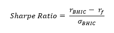
where the r’s stand for returns for BHIC and the risk-free return, respectively, and the sigma stands for the standard deviation of our returns. The higher the Sharpe ratio, the better the portfolio performed. We can compare our Sharpe Ratio with that of the S&P 500 Index in order to determine whether we outperformed or underperformed over the time period under analysis. Using the Sharpe ratio, it is clear there are only three ways to improve the portfolio’s risk-adjusted returns: increasing returns (assuming risk is constant), or decreasing risk (assuming returns are constant), or increasing returns while reducing risk.

Another method we can use to compare our overall risk-adjusted performance to the S&P 500 is Jensen’s alpha, which is rooted in the Capital Asset Pricing Model (CAPM) we use to calculate costs of capital for DDM and DCF models. The equation for Jensen’s alpha is as follows:

where each of the r’s stand for returns, from BHIC (BHIC), risk-free security (f), and the S&P 500 (m), and the beta used is the beta for our BHIC portfolio. In this model, CAPM is used as a way to calculate an expected return for our portfolio based on its risk. As applied in other analyses, the difference between the S&P’s return and the risk-free rate (proxied by the 10-year US treasury bond) is our risk premium. The risk premium is weighted by the beta computed for our portfolio. If our portfolio is more risky than the overall market, then the model will expect us to generate higher returns than the S&P.

The risk component of our expected return is added back to the risk-free rate to find our overall expected return. Finally, we subtract our expected return from our actual return, to find our alpha. If we achieve a positive alpha, it means we have beaten our benchmark on a risk-adjusted basis.

There are three ways to achieve positive alpha: by earning higher returns than the S&P with a beta of 1 (identical volatility to the S&P), by earning an identical return to the S&P with a beta lower than 1 (less volatility than the S&P), or by beating the market on both metrics at the same time. It is worth noting that positive alpha is extremely difficult to obtain on a consistent basis.